Pythonには,あらかじめ組み込まれている標準ライブラリと,別途インストールが必要なライブラリ(サードパーティライブラリ) がある。Pythonを使う上で極めて強力な数値計算ライブラリであるNumpyや,ポスト処理で必須なmatplotlibなどはすべてサードパーティーライブラリである。それらを個別にインストールしていくのはいささか面倒な作業であるので,科学技術計算に必要な多くのPython モジュールを含んだAnaconda を利用することを推奨する。Anacondaとは,Python 本体に加え,科学技術,数学,エンジニアリング,データ分析など,よく利用されるPython モジュール(2018 年10 月時点で800 以上)を一括でインストール可能にした総合パッケージであり,次のサイトからダウンロードできる。 https://www.anaconda.com/download/
以下,2018年10月時点におけるインストールの手順を簡単に説明する(※筆者はmacを一切使わないため以下はwindows前提の説明)。
-
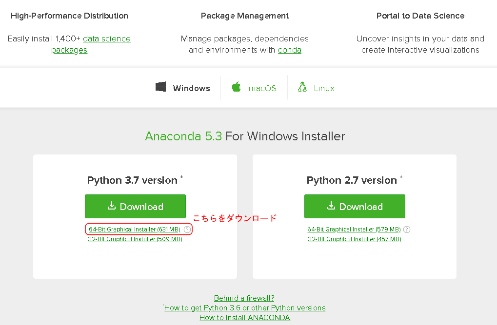
Anacondaのダウンロードサイトにアクセスし,windows64bit版をダウンロードする。
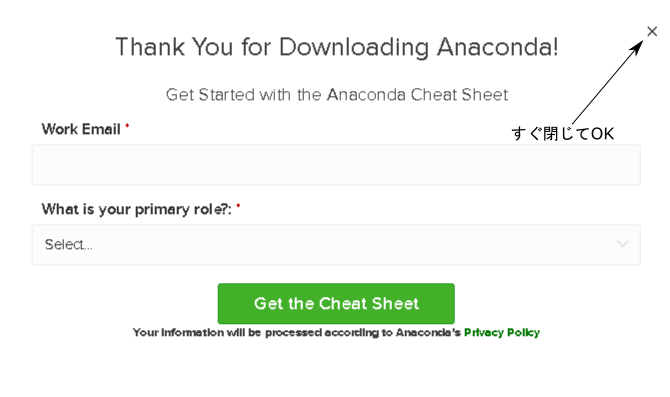
下記のようなポップアップが出るが,登録しなくてもダウンロードは進むので,無視して閉じて良い。
-
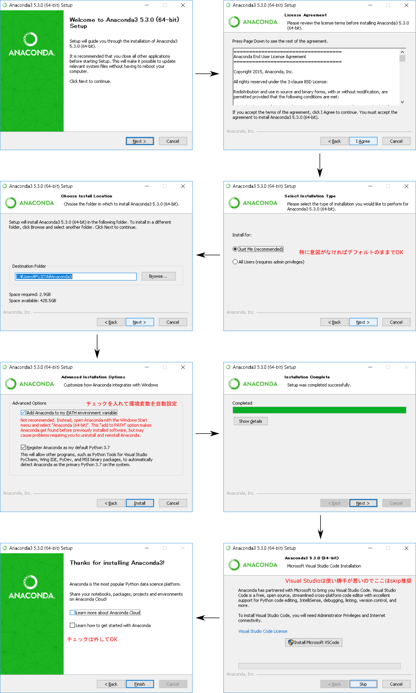
ダウンロードしたexeファイルをダブルクリックし,インストールを開始する(結構時間がかかります)。
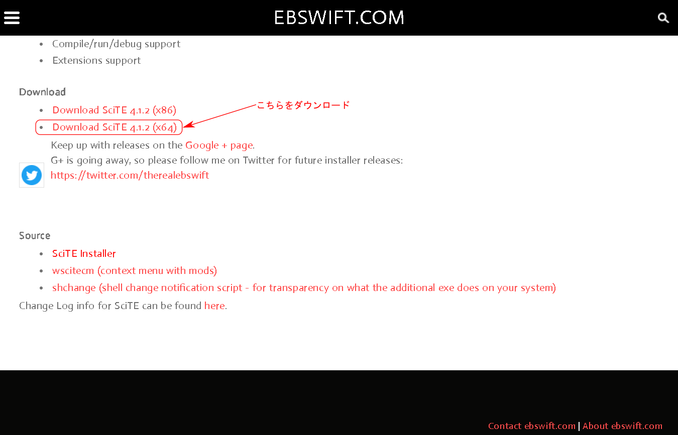
Pythonコードを編集するエディタはいくつかあるが,オススメのエディタの1つにSciTEがある。 Windows用にインストーラーが用意されおり,次のサイトからダウンロードできる。 https://www.ebswift.com/scite-text-editor-installer.html
以下,2018年10月時点におけるインストールの手順を簡単に説明する(※筆者はmacを一切使わないため以下はwindows前提の説明)。
-
SciTEのダウンロードサイトにアクセスし,ページ下部よりwindows64bit版をダウンロードする。
-
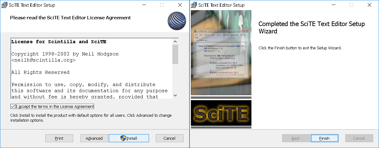
ダウンロードしたexeファイルをダブルクリックし,インストールを開始する。
-
このままでも十分実用に耐えるが,Pythonコードを書きやすくするためにいくつかカスタマイズが必要である。藤田が普段使用している独自にカスタマイズ済の設定ファイルを以下に示す(なお,藤田は本ホームページの編集もSciTEでおこなっています)。
locale.properties
others.properties
SciTEGlobal.properties
python.properties
html.properties
まず,上記のファイルをダウンロード(右クリック→名前を付けてリンク先を保存)し,C:\ProgramData\SciTE\に上書きコピーする。
次に以下のユーザーファイル
SciTEUser.properties
を,C:\Users\ユーザー名\AppData\Roaming\SciTE\に上書きコピーする。 以上の操作をおこなえば,背景が濃緑で見やすく色分けされたPythonコード表示が可能となる。
pyOpt( Python-based package for formulating and solving nonlinear constrained optimization problems)は,Python専用に設計されたフリーの最適化ライブラリ群であり,数理計画法からヒューリスティクスはまで幅広い最適化アルゴリズムを網羅している。残念ながら,開発自体は20014年でストップしており,元ソースはPython2.7以下までにしか対応していないが,Python3系でも使用できるように藤田が改良したソースをここに公開するので,こちらをbuild&installすればPython3以降でも使用することが可能となる。
pyOptはソースコードを直接buildする作業が必要となり,インストールの難易度は高い。1つずつ順を追って説明していく。
まず,インストール前の準備段階として,fortranコンパイラとswigを導入する必要がある。いずれも,condaでインストールできる。
-
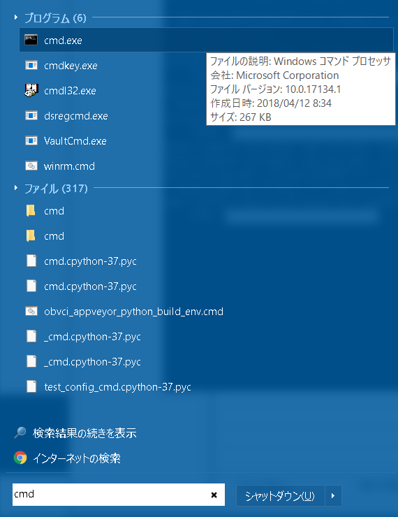
DOS画面を開く(スタートメニューで"cmd"と検索してEnterを押せばOK)。
-
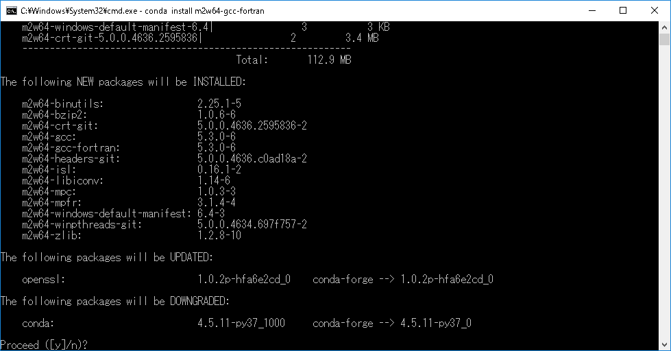
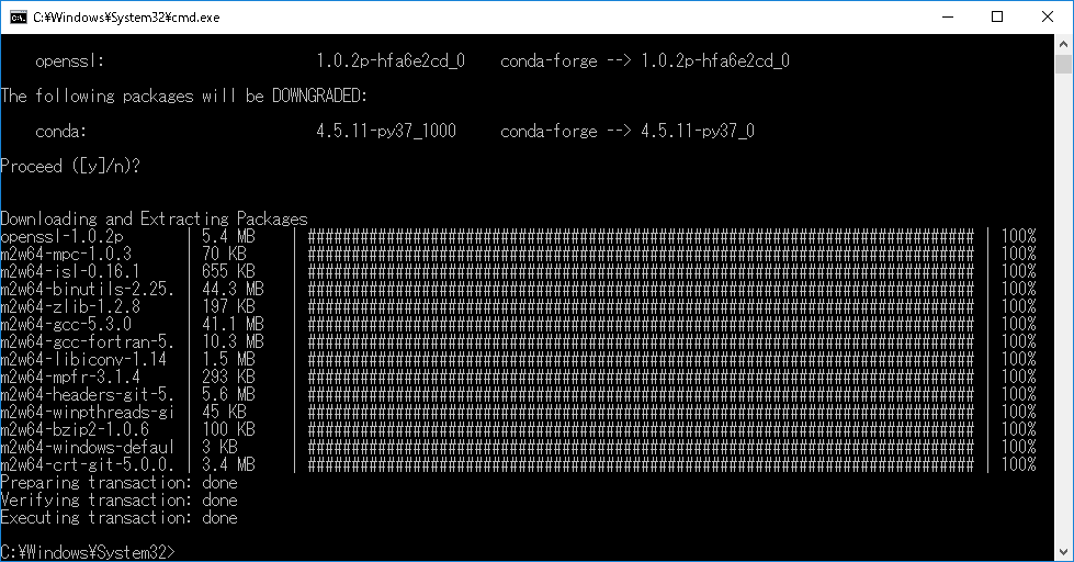
DOS画面にてconda install m2w64-gcc-fortranとタイプしEnter。

-
YesかNoか聞かれるのでyとタイプしEnter。
-
以上の操作でfortranコンパイラのインストールは終了。
-
DOS画面を開く(スタートメニューで"cmd"と検索してEnterを押せばOK)。
-
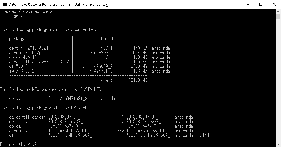
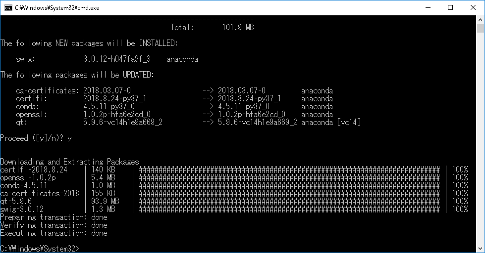
DOS画面にてconda install -c anaconda swigとタイプしEnter。

-
YesかNoか聞かれるのでyとタイプしEnter。
-
以上の操作でswigのインストールは終了。
-
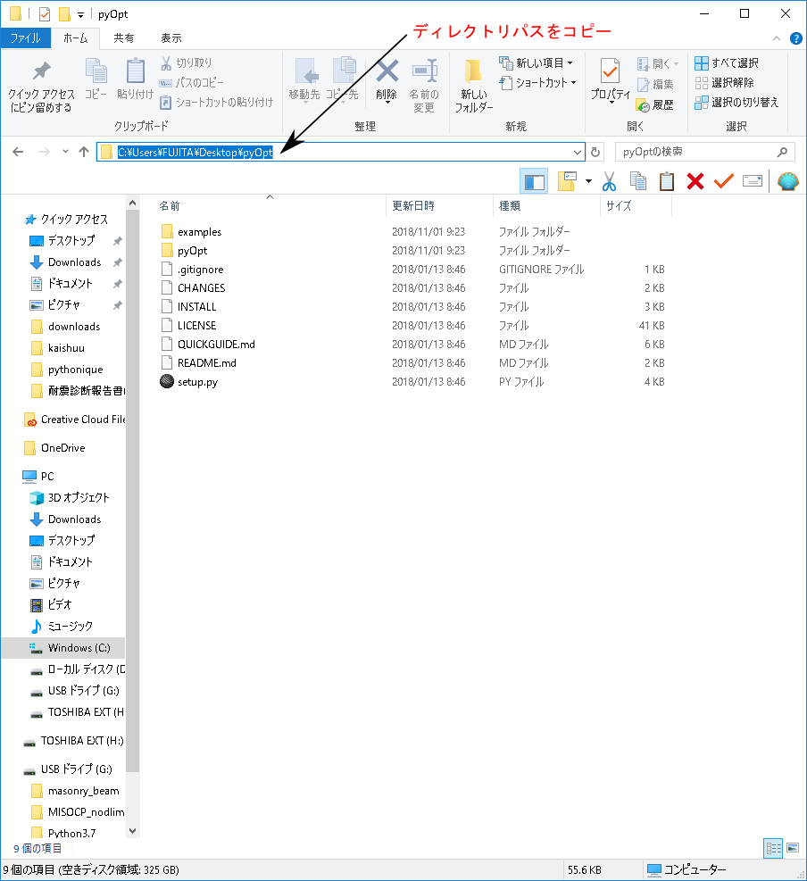
まず,藤田が独自に改良したPython3対応のpyOptをここからダウンロードする
(※研究室の学生は,更に改良を加えたこちらをダウンロードする)。
-
ダウンロードしたファイルを展開し,ディレクトリパスをコピーする。
-
DOS画面を開く(スタートメニューで"cmd"と検索してEnterを押せばOK)。
-
DOS画面にてcd 先ほどのディレクトリパスとタイプしEnter(pyOptディレクトリへの移動)。

-
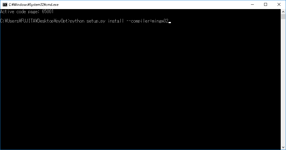
DOS画面にてchcp 65001とタイプしEnter(文字コードをSHIFT-JISからUTF-8に変更する操作)。

-
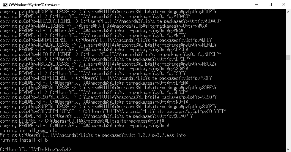
DOS画面にてpython setup.py install --compiler=mingw32とタイプしEnter。
-
以上の操作でpyOptのインストールは終了。
上記を解く以下のプログラムを実行し,結果が正しいことを確かめる(ソースはpyOptのexample内にある)。
tp037.py
#!/usr/bin/env python
'''
Solves Schittkowski's TP37 Constrained Problem.

    min 	-x1*x2*x3
    s.t.:	x1 + 2.*x2 + 2.*x3 - 72 <= 0
            - x1 - 2.*x2 - 2.*x3 <= 0
            0 <= xi <= 42,  i = 1,2,3

    f* = -3456 , x* = [24, 12, 12]
'''

# =============================================================================
# Standard Python modules
# =============================================================================
import os, sys, time
import pdb

# =============================================================================
# Extension modules
# =============================================================================
#from pyOpt import *
from pyOpt import Optimization
from pyOpt import PSQP
from pyOpt import SLSQP
from pyOpt import CONMIN
from pyOpt import COBYLA
from pyOpt import SOLVOPT
from pyOpt import KSOPT
from pyOpt import NSGA2
from pyOpt import ALGENCAN
from pyOpt import FILTERSD


# =============================================================================
#
# =============================================================================
def objfunc(x):

    f = -x[0]*x[1]*x[2]
    g = [0.0]*2
    g[0] = x[0] + 2.*x[1] + 2.*x[2] - 72.0
    g[1] = -x[0] - 2.*x[1] - 2.*x[2]

    fail = 0
    return f,g, fail


# =============================================================================
#
# =============================================================================

# Instantiate Optimization Problem
opt_prob = Optimization('TP37 Constrained Problem',objfunc)
opt_prob.addVar('x1','c',lower=0.0,upper=42.0,value=10.0)
opt_prob.addVar('x2','c',lower=0.0,upper=42.0,value=10.0)
opt_prob.addVar('x3','c',lower=0.0,upper=42.0,value=10.0)
opt_prob.addObj('f')
opt_prob.addCon('g1','i')
opt_prob.addCon('g2','i')
print opt_prob

# Instantiate Optimizer (PSQP) & Solve Problem
psqp = PSQP()
psqp.setOption('IPRINT',0)
psqp(opt_prob,sens_type='FD')
print(opt_prob.solution(0))

# Instantiate Optimizer (SLSQP) & Solve Problem
slsqp = SLSQP()
slsqp.setOption('IPRINT',-1)
slsqp(opt_prob,sens_type='FD')
print(opt_prob.solution(1))

# Instantiate Optimizer (CONMIN) & Solve Problem
conmin = CONMIN()
conmin.setOption('IPRINT',0)
conmin(opt_prob,sens_type='CS')
print(opt_prob.solution(2))

# Instantiate Optimizer (COBYLA) & Solve Problem
cobyla = COBYLA()
cobyla.setOption('IPRINT',0)
cobyla(opt_prob)
print(opt_prob.solution(3))

# Instantiate Optimizer (SOLVOPT) & Solve Problem
solvopt = SOLVOPT()
solvopt.setOption('iprint',-1)
solvopt(opt_prob,sens_type='FD')
print(opt_prob.solution(4))

# Instantiate Optimizer (KSOPT) & Solve Problem
ksopt = KSOPT()
ksopt.setOption('IPRINT',0)
ksopt(opt_prob,sens_type='FD')
print(opt_prob.solution(5))

# Instantiate Optimizer (NSGA2) & Solve Problem
nsga2 = NSGA2()
nsga2.setOption('PrintOut',0)
nsga2(opt_prob)
print(opt_prob.solution(6))

# Instantiate Optimizer (ALGENCAN) & Solve Problem
algencan = ALGENCAN()
algencan.setOption('iprint',0)
algencan(opt_prob)
print(opt_prob.solution(7))

# Instantiate Optimizer (FILTERSD) & Solve Problem
filtersd = FILTERSD()
filtersd.setOption('iprint',0)
filtersd(opt_prob)
print opt_prob.solution(8)
このプログラムを実行すると,pyOptが正しくインストールされていれば以下の出力が得られる。
Optimization Problem -- TP37 Constrained Problem
================================================================================

        Objective Function: objfunc

    Objectives:
        Name        Value        Optimum
	     f               0             0

	Variables (c - continuous, i - integer, d - discrete):
        Name    Type       Value       Lower Bound  Upper Bound
	     x1       c	     10.000000       0.00e+00     4.20e+01
	     x2       c	     10.000000       0.00e+00     4.20e+01
	     x3       c	     10.000000       0.00e+00     4.20e+01

	Constraints (i - inequality, e - equality):
        Name    Type                    Bounds
	     g1   	  i       -1.00e+21 <= 0.000000 <= 0.00e+00
	     g2   	  i       -1.00e+21 <= 0.000000 <= 0.00e+00


PSQP Solution to TP37 Constrained Problem
================================================================================

        Objective Function: objfunc

    Solution:
--------------------------------------------------------------------------------
    Total Time:                    0.0010
    Total Function Evaluations:        42
    Sensitivities:        FD

    Objectives:
        Name        Value        Optimum
	     f           -3456             0

	Variables (c - continuous, i - integer, d - discrete):
        Name    Type       Value       Lower Bound  Upper Bound
	     x1       c	     24.000000       0.00e+00     4.20e+01
	     x2       c	     12.000000       0.00e+00     4.20e+01
	     x3       c	     12.000000       0.00e+00     4.20e+01

	Constraints (i - inequality, e - equality):
        Name    Type                    Bounds
	     g1   	  i       -1.00e+21 <= 0.000000 <= 0.00e+00
	     g2   	  i       -1.00e+21 <= -72.000000 <= 0.00e+00

--------------------------------------------------------------------------------


SLSQP Solution to TP37 Constrained Problem
================================================================================

        Objective Function: objfunc

    Solution:
--------------------------------------------------------------------------------
    Total Time:                    0.0010
    Total Function Evaluations:         0
    Sensitivities:        FD

    Objectives:
        Name        Value        Optimum
	     f           -3456             0

	Variables (c - continuous, i - integer, d - discrete):
        Name    Type       Value       Lower Bound  Upper Bound
	     x1       c	     24.000000       0.00e+00     4.20e+01
	     x2       c	     12.000000       0.00e+00     4.20e+01
	     x3       c	     12.000000       0.00e+00     4.20e+01

	Constraints (i - inequality, e - equality):
        Name    Type                    Bounds
	     g1   	  i       -1.00e+21 <= 0.000000 <= 0.00e+00
	     g2   	  i       -1.00e+21 <= -72.000000 <= 0.00e+00

--------------------------------------------------------------------------------


CONMIN Solution to TP37 Constrained Problem
================================================================================

        Objective Function: objfunc

    Solution:
--------------------------------------------------------------------------------
    Total Time:                    0.0010
    Total Function Evaluations:        88
    Sensitivities:        CS

    Objectives:
        Name        Value        Optimum
	     f           -3456             0

	Variables (c - continuous, i - integer, d - discrete):
        Name    Type       Value       Lower Bound  Upper Bound
	     x1       c	     23.989921       0.00e+00     4.20e+01
	     x2       c	     12.002518       0.00e+00     4.20e+01
	     x3       c	     12.002518       0.00e+00     4.20e+01

	Constraints (i - inequality, e - equality):
        Name    Type                    Bounds
	     g1   	  i       -1.00e+21 <= -0.000006 <= 0.00e+00
	     g2   	  i       -1.00e+21 <= -71.999994 <= 0.00e+00

--------------------------------------------------------------------------------


COBYLA Solution to TP37 Constrained Problem
================================================================================

        Objective Function: objfunc

    Solution:
--------------------------------------------------------------------------------
    Total Time:                    0.0010
    Total Function Evaluations:       112

    Objectives:
        Name        Value        Optimum
	     f           -3456             0

	Variables (c - continuous, i - integer, d - discrete):
        Name    Type       Value       Lower Bound  Upper Bound
	     x1       c	     24.000000       0.00e+00     4.20e+01
	     x2       c	     11.999999       0.00e+00     4.20e+01
	     x3       c	     12.000000       0.00e+00     4.20e+01

	Constraints (i - inequality, e - equality):
        Name    Type                    Bounds
	     g1   	  i       -1.00e+21 <= 0.000000 <= 0.00e+00
	     g2   	  i       -1.00e+21 <= -72.000000 <= 0.00e+00

--------------------------------------------------------------------------------


SOLVOPT Solution to TP37 Constrained Problem
================================================================================

        Objective Function: objfunc

    Solution:
--------------------------------------------------------------------------------
    Total Time:                    0.0070
    Total Function Evaluations:       201
    Sensitivities:        FD

    Objectives:
        Name        Value        Optimum
	     f           -3456             0

	Variables (c - continuous, i - integer, d - discrete):
        Name    Type       Value       Lower Bound  Upper Bound
	     x1       c	     23.999011       0.00e+00     4.20e+01
	     x2       c	     12.000860       0.00e+00     4.20e+01
	     x3       c	     11.999634       0.00e+00     4.20e+01

	Constraints (i - inequality, e - equality):
        Name    Type                    Bounds
	     g1   	  i       -1.00e+21 <= -0.000000 <= 0.00e+00
	     g2   	  i       -1.00e+21 <= -72.000000 <= 0.00e+00

--------------------------------------------------------------------------------


KSOPT Solution to TP37 Constrained Problem
================================================================================

        Objective Function: objfunc

    Solution:
--------------------------------------------------------------------------------
    Total Time:                    0.0110
    Total Function Evaluations:      2187
    Sensitivities:        FD

    Objectives:
        Name        Value        Optimum
	     f        -3453.73             0

	Variables (c - continuous, i - integer, d - discrete):
        Name    Type       Value       Lower Bound  Upper Bound
	     x1       c	     23.995259       0.00e+00     4.20e+01
	     x2       c	     11.997588       0.00e+00     4.20e+01
	     x3       c	     11.996896       0.00e+00     4.20e+01

	Constraints (i - inequality, e - equality):
        Name    Type                    Bounds
	     g1   	  i       -1.00e+21 <= -0.015771 <= 0.00e+00
	     g2   	  i       -1.00e+21 <= -71.984229 <= 0.00e+00

--------------------------------------------------------------------------------


NSGA-II Solution to TP37 Constrained Problem
================================================================================

        Objective Function: objfunc

    Solution:
--------------------------------------------------------------------------------
    Total Time:                    0.0688
    Total Function Evaluations:         0

    Objectives:
        Name        Value        Optimum
	     f        -3455.25             0

	Variables (c - continuous, i - integer, d - discrete):
        Name    Type       Value       Lower Bound  Upper Bound
	     x1       c	     24.259110       0.00e+00     4.20e+01
	     x2       c	     11.858676       0.00e+00     4.20e+01
	     x3       c	     12.010719       0.00e+00     4.20e+01

	Constraints (i - inequality, e - equality):
        Name    Type                    Bounds
	     g1   	  i       -1.00e+21 <= -0.002100 <= 0.00e+00
	     g2   	  i       -1.00e+21 <= -71.997900 <= 0.00e+00

--------------------------------------------------------------------------------


ALGENCAN Solution to TP37 Constrained Problem
================================================================================

        Objective Function: objfunc

    Solution:
--------------------------------------------------------------------------------
    Total Time:                    0.0030
    Total Function Evaluations:         0
    Lambda: [144.00000063   0.        ]
    Sensitivities:        FD

    Objectives:
        Name        Value        Optimum
	     f           -3456             0

	Variables (c - continuous, i - integer, d - discrete):
        Name    Type       Value       Lower Bound  Upper Bound
	     x1       c	     24.000000       0.00e+00     4.20e+01
	     x2       c	     12.000000       0.00e+00     4.20e+01
	     x3       c	     12.000000       0.00e+00     4.20e+01

	Constraints (i - inequality, e - equality):
        Name    Type                    Bounds
	     g1   	  i       -1.00e+21 <= 0.000000 <= 0.00e+00
	     g2   	  i       -1.00e+21 <= -72.000000 <= 0.00e+00

--------------------------------------------------------------------------------


FILTERSD Solution to TP37 Constrained Problem
================================================================================

        Objective Function: objfunc

    Solution:
--------------------------------------------------------------------------------
    Total Time:                    0.0010
    Total Function Evaluations:        69
    Lambda:   [0. 0.]
    Sensitivities:        FD

    Objectives:
        Name        Value        Optimum
	     f           -3456             0

	Variables (c - continuous, i - integer, d - discrete):
        Name    Type       Value       Lower Bound  Upper Bound
	     x1       c	     24.000000       0.00e+00     4.20e+01
	     x2       c	     12.000000       0.00e+00     4.20e+01
	     x3       c	     12.000000       0.00e+00     4.20e+01

	Constraints (i - inequality, e - equality):
        Name    Type                    Bounds
	     g1   	  i       -1.00e+21 <= 0.000000 <= 0.00e+00
	     g2   	  i       -1.00e+21 <= -72.000000 <= 0.00e+00

--------------------------------------------------------------------------------
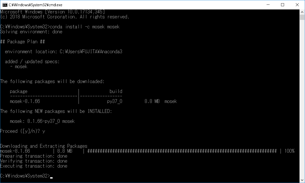
混合整数計画問題をはじめとした高度な最適化問題を理論的に解く強力な商用ソルバーの1つにMosekがある。 アカデミックユーズであれば無料で使用することができ,Pythonとの親和性が極めて高く,condaを使ってインストールできる。 以下,2018年10月時点におけるインストールの手順を簡単に説明する(※筆者はmacを一切使わないため以下はwindows前提の説明)。
-
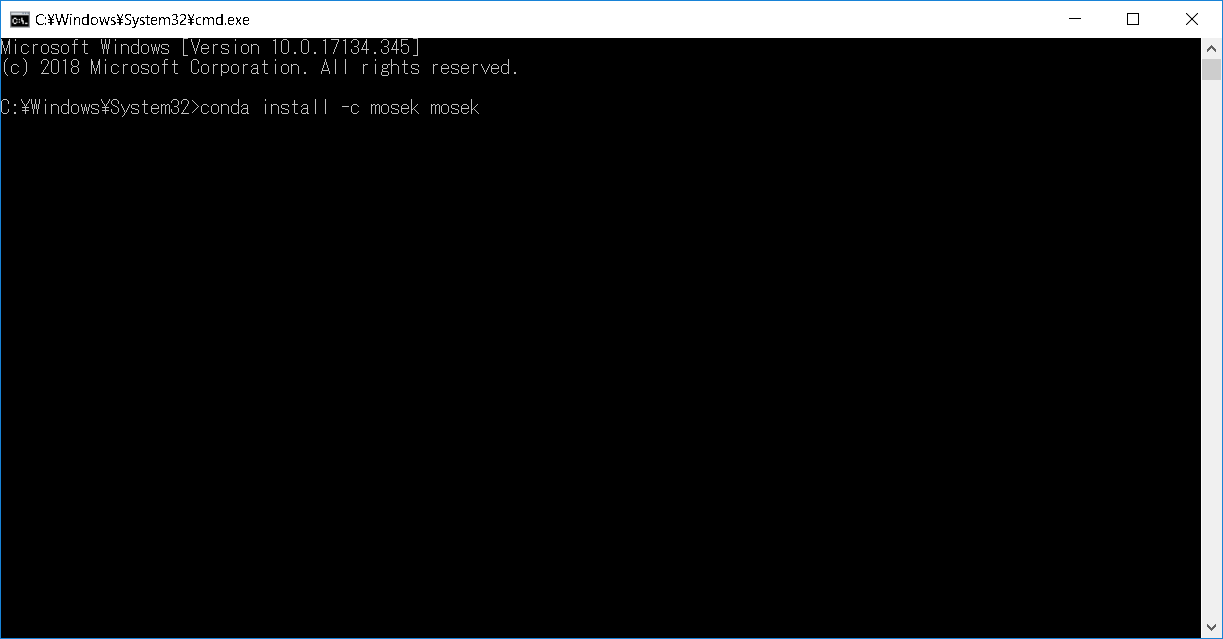
DOS画面を開く(スタートメニューで"cmd"と検索してEnterを押せばOK)。
-
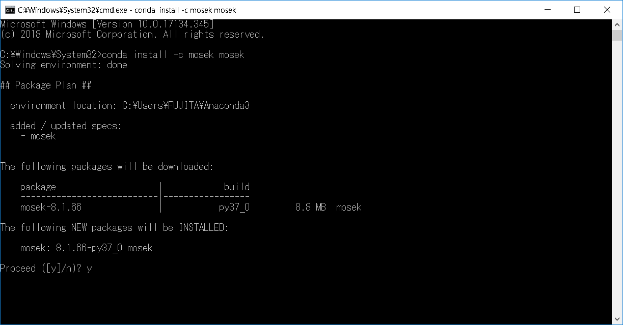
DOS画面にてconda install -c mosek mosekとタイプしEnter。
-
YesかNoか聞かれるのでyとタイプしEnter。
-
以上の操作でインストールは終了。
以下,ライセンスの登録手順を説明する。
-
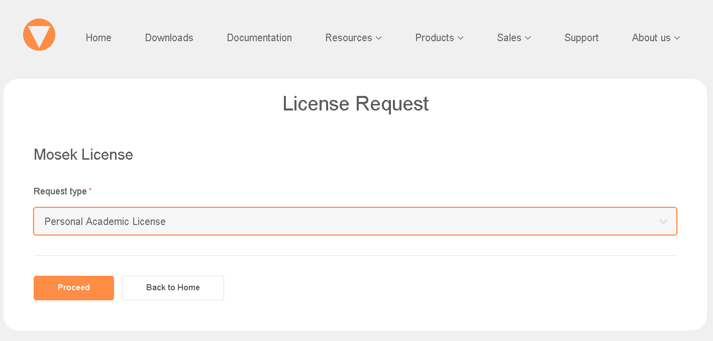
ダウンロードサイトで"Request Personal Academic License"をクリック。

-
選択が"Personal Academic License"になっていることを確認し,"Proceed"をクリック。
-
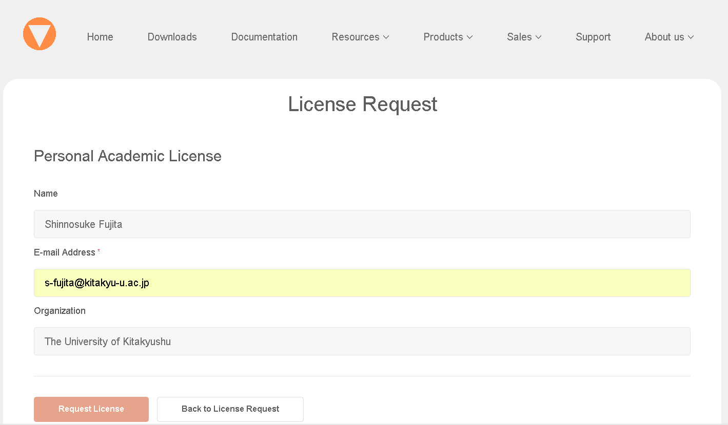
必要事項を入力し,"Request License"をクリック(ライセンスファイルは登録したメールアドレス宛に届く)。
-
正しく処理されれば,次のような画面に遷移しますので,"I Accept The License Agreement"をクリック。

-
登録したアドレス宛に mosek.lic というライセンスファイルが送られて来るので,これをダウンロードする。
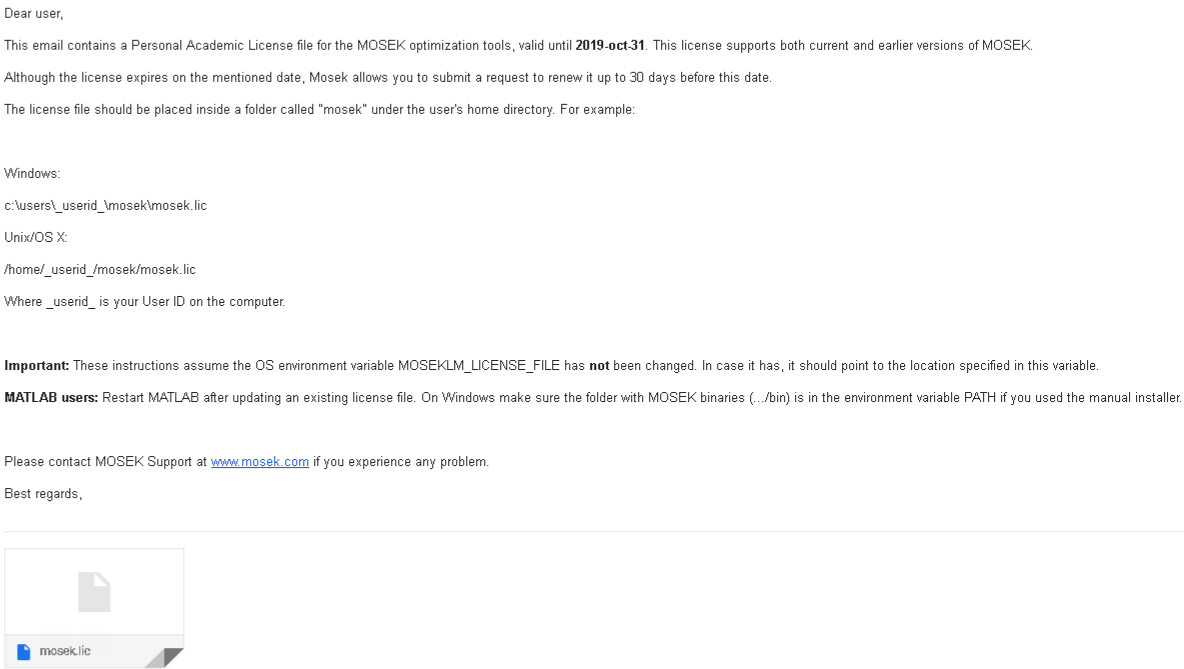
- ライセンスファイルを C:\Users\ユーザー名\mosek\ にコピーすればMosekが使えるようになる(ユーザー名以下にデフォルトではmosekというフォルダは存在しないので,新規作成する必要がある)。
-
DOS画面を開く(スタートメニューで"cmd"と検索してEnterを押せばOK)。
-
DOS画面にてpip install picosとタイプしEnter。

-
以上の操作でインストールは終了。
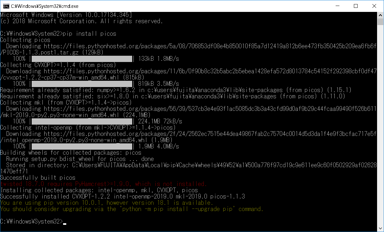
You are using pip version *****, however version ***** is available.
You should consider upgrading via the 'python -m pip install --upgrade pip' command
-
DOS画面を開く(スタートメニューで"cmd"と検索してEnterを押せばOK)。
-
DOS画面にてpython -m pip install --upgrade pipとタイプしEnter。
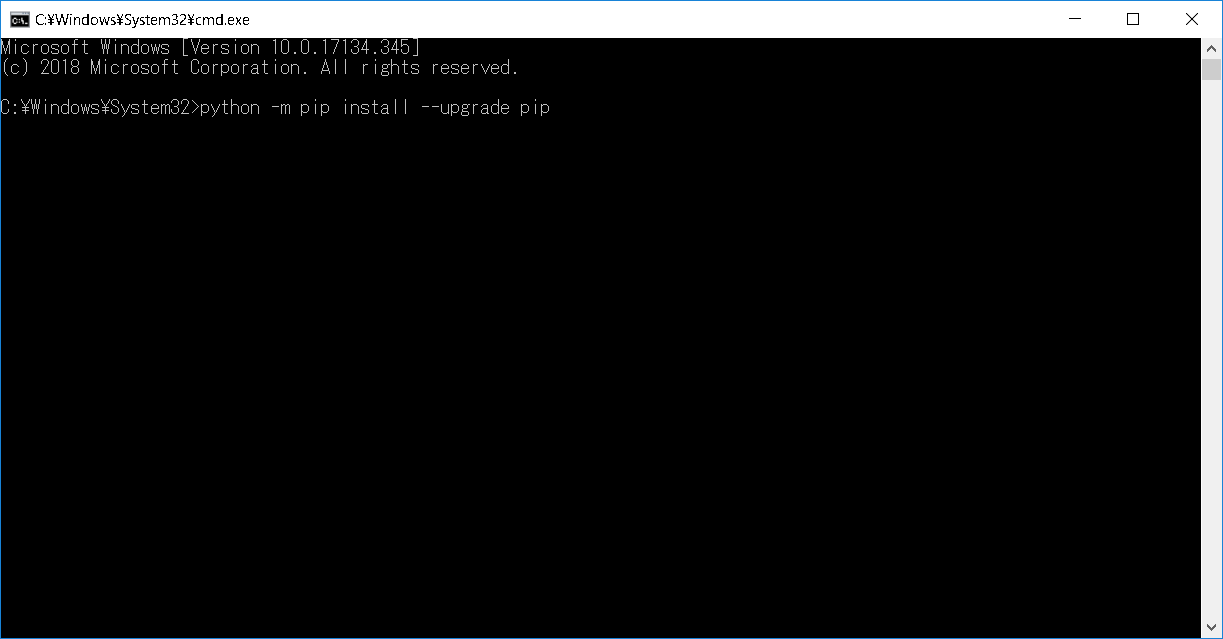
-
以上の操作でpipのアップデートは終了。
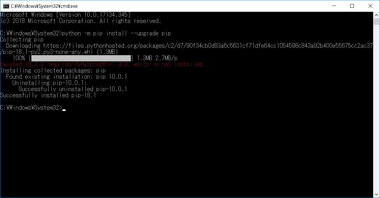
twisted 18.7.0 requires PyHamcrest>=1.9.0, which is not installed.
-
DOS画面を開く(スタートメニューで"cmd"と検索してEnterを押せばOK)。
-
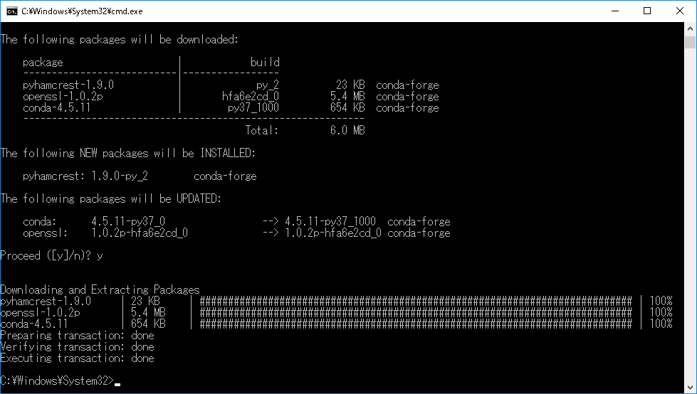
DOS画面にてconda install -c conda-forge pyhamcrestとタイプしEnter。
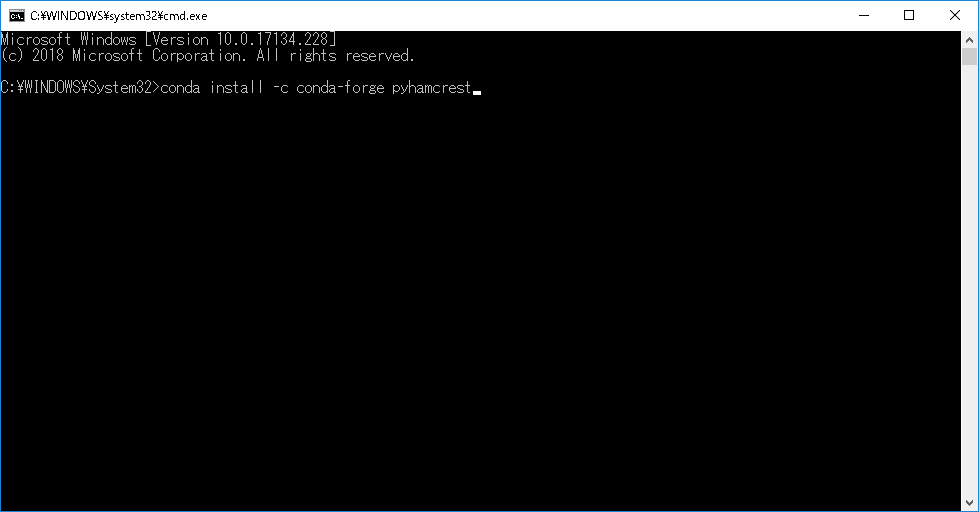
-
YesかNoか聞かれるのでyとタイプしEnter。
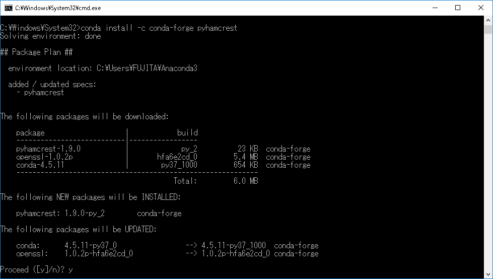
-
以上の操作でPyHamcrestのインストールは終了。
DOS画面にて以下のコマンドでインストールできる。
| OpenSeesPy(有限要素法) | pip install openseespy |
| VTK(可視化ライブラリ) | conda install -c anaconda vtk |
| Netgen(FEM用メッシュジェネレータ) | conda install -c conda-forge netgen |
| wxPython(GUI作成) | pip install wxpython |
matplotlibのデフォルトのフォント設定では,labelやtitleに日本語を使用すると文字化けしてしまう。 matplotlibで日本語を使用するには,日本語に対応したフォントを使用する必要がある。
matplotlibで使用できるフォントの一覧は以下のコードで確認することができる。
import matplotlib.font_manager as fm

fonts=fm.findSystemFonts()
for font in fonts:print(fm.FontProperties(fname=font).get_name())
HGMaruGothicMPRO
IPAexGothic
Malgun Gothic
HGSeikaishotaiPRO
気に入ったフォントが見つからない場合は,外部からダウンロードしてくると良い。matplotlib対応の日本語フリーフォントで有名なものとして,IPAexフォントがある。 ここからダウンロードできる。ダウンロードしたファイルを解凍するとipaexg.ttfというTrueTypeフォントファイルがあるので,それを'lib\\site-packages\\matplotlib\\mpl-data\\fonts'以下にコピーすれば使用できるようになる。
使用する日本語フォントを決めたら,プログラム上で呼び出す。matplotlibで使用するすべてのフォントを一括で指定する場合は, プログラムの冒頭で次のように記述すればよい。
import matplotlib.pyplot as plt

plt.rcParams['font.family'] = 'IPAexGothic' #全体のフォントを設定
一方で,グラフの特定の文字のみフォントを変更したい場合は,次のようにすると良い。
ax.set_title('title',**{'family':'IPAexGothic'}) #タイトルのフォントのみをIPAexGothicに指定
ax.set_xlabel('x label',**{'family':'IPAexGothic'}) #X軸ラベルのフォントのみをIPAexGothicに指定
毎回のプログラムソースの中でフォントを指定するのは面倒だという場合は,matplotlibの設定ファイルを編集してデフォルトのフォント自体を変更することもできる。 デフォルトでは,'lib\\site-packages\\matplotlib\\mpl-data\\matplotlibrc'に設定ファイルがある。 この設定ファイルを直接編集しても良いのだが,編集を誤った時にmatplotlibが正しく動作しなくなる恐れがあるので, これを'C:\Users\your_name\.matplotlib\'以下にコピー&ペーストそちらを編集する方が無難。 'C:\Users\your_name\.matplotlib\matplotlibrc'をテキストエディタで開くと,196行目付近に
# The font.size property is the default font size for text, given in pts.
# 10 pt is the standard value.
#
font.family         : sans-serif
#font.style          : normal
#font.variant        : normal
#font.weight         : medium
#font.stretch        : normal
# The font.size property is the default font size for text, given in pts.
# 10 pt is the standard value.
#
#font.family         : sans-serif
font.family           : IPAexGothic
#font.style          : normal
#font.variant        : normal
#font.weight         : medium
#font.stretch        : normal
import matplotlib
print(matplotlib.matplotlib_fname())
ファイルの入出力を行う場合,EXCELとの親和性の高さを考えれば,csvファイルとして入出力を行うと良い。
例えば次のようなcsvファイル test.csv がソースと同じディレクトリの datain というフォルダに用意されているとする。
test.csv
X,Y,Z
0,0,0
1,1,1
2,2,2
,,
I,J,
0,1,
1,2,
import csv

filename='test.csv'
foldername='datain'
reader=csv.reader(open(foldername+'/'+filename))
r,ij=[],[] #rとijのリスト定義

next(reader) #ラベル行を読み飛ばす
for row in reader:
	if row[0]=='': break #空欄になるまで読み込む
	r.append([float(row[0]),float(row[1]),float(row[2])]) #座標を実数として読み込み

next(reader) #ラベル行を読み飛ばす
for row in reader:
	if row[0]=='': break #空欄になるまで読み込む
	ij.append([int(row[0]),int(row[1])]) #要素節点関係を整数として読み込み

print(r) #試しに出力してみる
print(ij) #試しに出力してみる
[[0.0, 0.0, 0.0], [1.0, 1.0, 1.0], [2.0, 2.0, 2.0]]
[[0, 1], [1, 2]]
今度は逆に,python内の数値データをcsvファイルとして出力する場合を考える。 先ほどのプログラムの続きに,以下のコードを追記してみよう。
import os

output_filename='test2.csv'
output_foldername='dataout'
try:os.stat(output_foldername)#dataoutという名前のフォルダの有無を調査
except:os.mkdir(output_foldername)#なければ新規にdataoutという名前のフォルダを作成する
writer=csv.writer(open(output_foldername+'/'+output_filename,'w',newline=''))

writer.writerow(['X','Y','Z']) #ラベル行を出力
for ri in r:
	writer.writerow([ri[0],ri[1],ri[2]]) #rの値を1行ずつ出力
writer.writerow(['','','']) #改行

writer.writerow(['I','J']) #ラベル行を出力
for eij in ij:
	writer.writerow([eij[0],eij[1]]) #ijの値を1行ずつ出力
test2.csv
X,Y,Z
0.0,0.0,0.0
1.0,1.0,1.0
2.0,2.0,2.0
,,
I,J
0,1
1,2
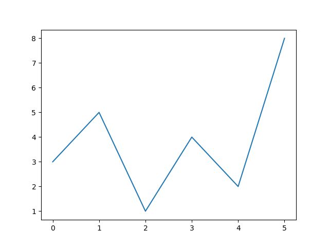
pythonにはmatplotlibというグラフ描画のための強力なライブラリがあり,これを用いれば科学技術計算分野で必要とされるグラフのほとんどを表現することができる。 折れ線グラフを描画する最もシンプルなプログラムは以下の通り。
import matplotlib.pyplot as plt #2次元グラフ描画のためのモジュールの読み込み

x=[0,1,2,3,4,5] #x座標
y=[3,5,1,4,2,8] #y座標
plt.plot(x,y) #グラフの書込み

plt.show() #描画
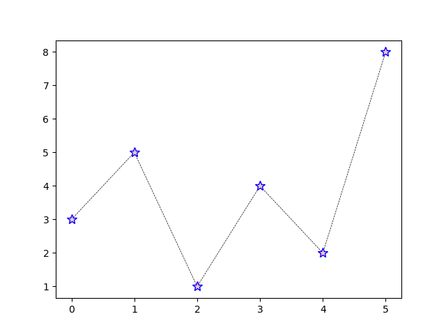
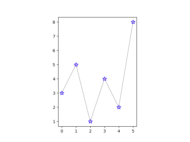
import matplotlib.pyplot as plt #2次元グラフ描画のためのモジュールの読み込み

x=[0,1,2,3,4,5] #x座標
y=[3,5,1,4,2,8] #y座標
plt.plot(x,y,linestyle='dashed',linewidth=0.5,color='black',
marker='*',markeredgewidth=1,markeredgecolor='blue',
markersize=10,markerfacecolor='pink') #グラフの書込み(描画オプション付き)

plt.show() #描画
import matplotlib.pyplot as plt #2次元グラフ描画のためのモジュールの読み込み

x=[0,1,2,3,4,5] #x座標
y=[3,5,1,4,2,8] #y座標

plt.axes().set_aspect('equal') #縦横比を揃える

plt.plot(x,y,linestyle='dashed',linewidth=0.5,color='black',
marker='*',markeredgewidth=1,markeredgecolor='blue',
markersize=10,markerfacecolor='pink') #グラフの書込み(描画オプション付き)

plt.show() #描画
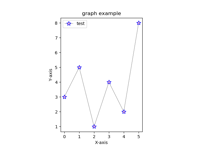
import matplotlib.pyplot as plt #2次元グラフ描画のためのモジュールの読み込み

x=[0,1,2,3,4,5] #x座標
y=[3,5,1,4,2,8] #y座標

plt.axes().set_aspect('equal') #縦横比を揃える

plt.plot(x,y,linestyle='dashed',linewidth=0.5,color='black',
marker='*',markeredgewidth=1,markeredgecolor='blue',
markersize=10,markerfacecolor='pink',label='test') #グラフの書込み(描画オプション付き)

plt.title('graph example') #グラフタイトル
plt.xlabel('X-axis') #X軸ラベル
plt.ylabel('Y-axis') #Y軸ラベル
plt.legend() #凡例の描画(plt.plotでlabelを指定する必要がある)

plt.show() #描画
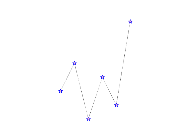
import matplotlib.pyplot as plt #2次元グラフ描画のためのモジュールの読み込み

x=[0,1,2,3,4,5] #x座標
y=[3,5,1,4,2,8] #y座標

plt.axes().set_aspect('equal') #縦横比を揃える

plt.plot(x,y,linestyle='dashed',linewidth=0.5,color='black',
marker='*',markeredgewidth=1,markeredgecolor='blue',
markersize=10,markerfacecolor='pink',label='test') #グラフの書込み(描画オプション付き)

plt.tick_params(labelbottom=False,bottom=False) # x軸の削除
plt.tick_params(labelleft=False,left=False) # y軸の削除
plt.box(False) #枠の消去

plt.show() #描画